This blog post started as a “what if” contemplation in my head: Suppose you have a reasonably large table with a clustered index and a number of non-clustered indexes. If your WHERE clause filters by multiple columns covered by those non-clustered indexes, could it potentially be faster to rewrite that WHERE clause to use those non-clustered indexes?

The answer might surprise you.

Setup

Suppose we have this table with about 15 million of rows:

CREATE TABLE #tbl (
    pk          int IDENTITY(1, 1) NOT NULL,
    a           int NOT NULL,
    b           int NOT NULL,
    c           int NOT NULL,
    d           int NOT NULL,
    e           int NOT NULL,
    f           int NOT NULL,
    CONSTRAINT PK PRIMARY KEY CLUSTERED (pk),
    INDEX IX_a_b (a, b),
    INDEX IX_c_d (c, d),
    INDEX IX_e_f (e, f)
);

INSERT INTO #tbl (a, b, c, d, e, f)
VALUES (0, 1, 3, 2, 4, 5), (0, 1, 3, 2, 4, 5),
       (0, 1, 3, 2, 4, 5), (0, 1, 3, 2, 4, 5),
       (0, 1, 3, 2, 4, 5), (0, 1, 3, 2, 4, 5),
       (0, 1, 3, 2, 4, 5), (0, 1, 3, 2, 4, 5),
       (0, 1, 3, 2, 4, 5), (0, 1, 3, 2, 4, 5),
       (0, 1, 3, 2, 4, 5), (0, 1, 3, 2, 4, 5),
       (0, 1, 3, 2, 4, 5), (0, 1, 3, 2, 4, 5);

WHILE (@@ROWCOUNT<5000000)
    INSERT INTO #tbl (a, b, c, d, e, f)
    SELECT a+1, b+1, c+1428, d+1, e+10, (f+1)%10
    FROM #tbl;

.. and we want this query to perform optimally:

SELECT t1.*
FROM #tbl AS t1
WHERE t1.a IN (1, 2, 3, 4, 5)
  AND t1.c=9999
  AND t1.e>100 AND t1.f=2;

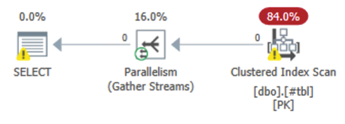
The Clustered Index Scan

I bet the most common plan you’ll see for a query that looks like this is a simple clustered index scan. Because the clustered index contains all of the columns, and because our WHERE criteria covers columns a, c, e and f. No single non-clustered index would do a great job here.

As the name “scan” implies, the Clustered Index Scan will read through every row in the table and select those that match the WHERE clause (also called the “predicate”).

The plan contains absolutely zero surprises.

You could force this plan by adding an index hint:

SELECT t1.*
FROM #tbl AS t1 WITH (INDEX=1)
WHERE t1.a IN (1, 2, 3, 4, 5)
  AND t1.c=9999
  AND t1.e>100 AND t1.f=2;

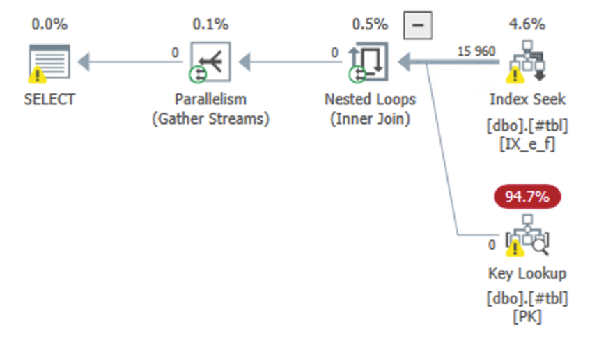
The Key Lookup

You’ve already seen Key Lookups many, many times. SQL Server uses statistics to look for a column and index that will yield the fewest number of rows given the WHERE clause we’re using, and then performs a seek on that non-clustered index. Hopefully, it returns only a handful of rows, so we can run a Key Lookup to fetch the remaining columns.

You can force this plan using:

SELECT t1.*
FROM #tbl AS t1 WITH (INDEX=IX_e_f)
WHERE t1.a IN (1, 2, 3, 4, 5)
  AND t1.c=9999
  AND t1.e>100 AND t1.f=2;

This happens when at least one column has relatively unique values (a high selectivity), so that we can minimize the number of key lookups.

Piecing together multiple non-clustered indexes

Edit: I’ve learned from Kendra Little that this is called an “Index intersection”, which makes perfect sense.

Hear me out. Could we just use only non-clustered indexes? They’re smaller, but more importantly, they’re indexed so that we can perform index seeks (range scans, actually) to the exact values that we’re looking for, and then join those indexes together, so that should be much faster, right?

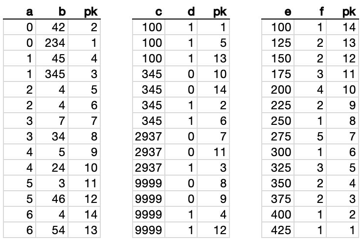
Think of every non-clustered index as a vertical subset of the table (in this case, just the index columns and the clustering key). More importantly, a non-clustered index is sorted by its index keys, which allows us to perform Index Seeks rather than Scans.

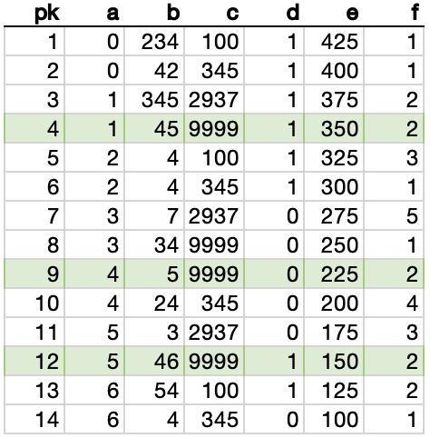
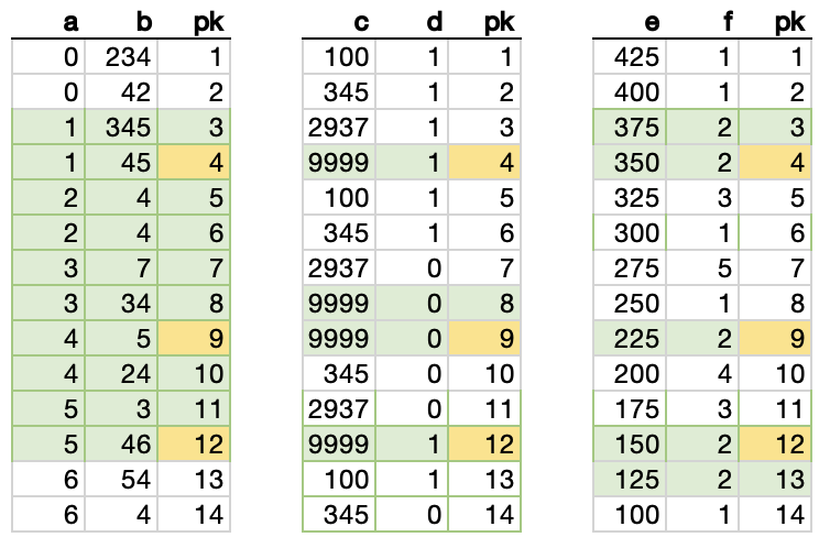
Here’s how the three non-clustered indexes on our table look:

So we could apply parts of the WHERE clause to each respective index…

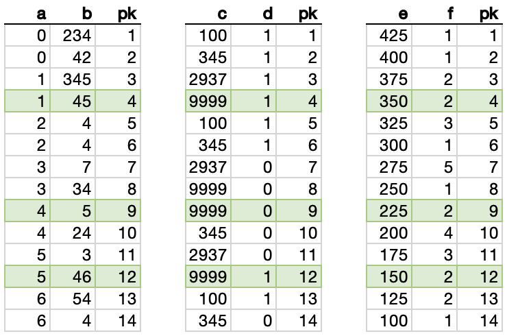
… and then INNER JOIN those three datasets using the “pk” column, which is present in all three:

Because our WHERE criteria is a series of AND conditions, we’re INNER JOINing these three sets, so we’re looking only for rows that are marked in green in all three sets.

Now, we can see the result of the join, which is the same result that we got from our original clustered index scan:

Here’s how that looks like in the execution plan:

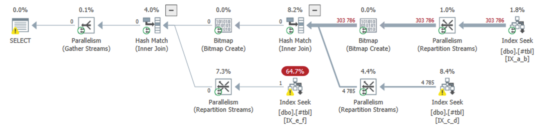
In terms of T-SQL, you could force this three-index join like this:

SELECT t1.pk, t1.a, t1.b, t2.c, t2.d, t3.e, t3.f
FROM #tbl AS t1 WITH (INDEX=IX_a_b)
INNER JOIN #tbl AS t2 WITH (INDEX=IX_c_d) ON t1.pk=t2.pk
INNER JOIN #tbl AS t3 WITH (INDEX=IX_e_f) ON t1.pk=t3.pk
WHERE t1.a IN (1, 2, 3, 4, 5)
  AND t2.c=9999
  AND t3.e>100 AND t3.f=2;

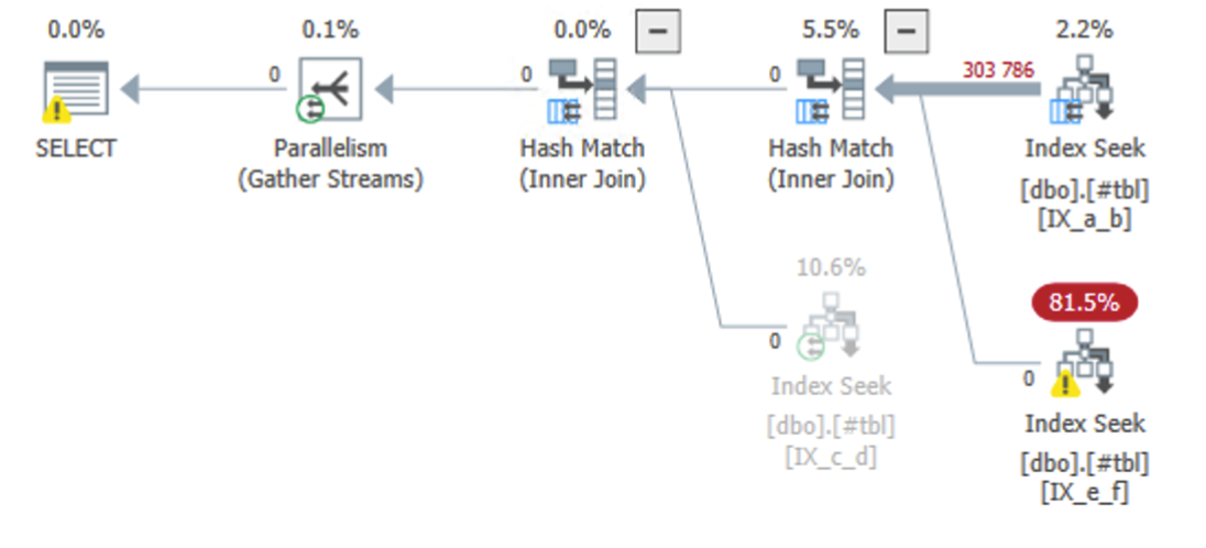
But forcing the indexes actually produces a slightly cleaner plan:

What determines what plan we get?

SQL Server uses statistics on the various indexes (rough guestimates of the data distribution and count) to determine which plan will work out best.

The Key Lookup is ideal when column predicate allows you to quickly filter down to just a handful of rows in one index. The important part here is the “just a handful” part – Key Lookups are relatively cheap when you do a few, and potentially terrible when you have to do millions of them.

The Non-clustered Index Seek joins works in a specific scenario where no single index can narrow down the rows enough to perform Key Lookups, but the Clustered Index Scan would be too wasteful because you’d have to scan the entire table.

The Clustered Index Scan is perfect when you’re likely to return a majority of the table anyway – no need to join anything.

Conclusions

I was already very familiar with the Clustered Index Scan and it’s slightly deranged cousin, the Key Lookup, but as I was playing around with the idea of manually joining multiple non-clustered indexes, I didn’t realize that there are cases where SQL Server will actually do this automatically.

Oh, and I also realized right after I’d finished this post that I’ve already written a similar one (albeit not exactly the same).