How to fix rounding errors

A number of business processes require you to distribute a value over a date range. However, if your distribution keys and values don’t add up perfectly or aren’t perfectly divisible, it’s very easy to get rounding errors in your distributions.

Demo setup

Here are 65,000 example balances that we’ll try to distribute over 12 months:

CREATE TABLE #balances (
    id          int NOT NULL,
    balance     numeric(12, 2) NOT NULL,
    PRIMARY KEY CLUSTERED (id)
);

--- Create four examples
INSERT INTO #balances
VALUES (1,    1.00),
       (2,  100.00),
       (3,  240.00),
       (4, 1000.00);

--- Duplicate the results
WHILE (@@ROWCOUNT<30000)
    INSERT INTO #balances
    SELECT MAX(id) OVER ()+id, balance
    FROM #balances;

We’ll also create a table that contains the distribution key that we want to apply. This one’s a simple straigh-line 12-month accrual, but you could put any distribution key in there as long as they add up to 1.0:

CREATE TABLE #distribution (
    [period]    tinyint NOT NULL,
    [key]       numeric(6, 6) NOT NULL,
    PRIMARY KEY CLUSTERED ([period])
);

INSERT INTO #distribution
SELECT [period], 1./12 AS [key]
FROM (
    VALUES (1), (2), (3), (4), (5), (6),
           (7), (8), (9), (10), (11), (12)
    ) AS x([period]);

A plain distribution will create rounding errors

This query will distribute the balances over the 12 months, turning the 65,000 rows into 786,000 ones:

SELECT bal.id,
       bal.balance,
       d.[period],
       CAST(bal.balance*d.[key] AS numeric(12, 2)) AS distributed_balance
FROM #balances AS bal
CROSS JOIN #distribution AS d;

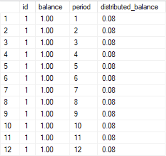
Because we’ve rounded the result of the distribution to the same precision as the balance, the resulting rows are 0.08 each. Add those up, and you get 0.96, not 1.00. Which may be fine if you’re working with geographical measurements, but not if you’re doing accounting.

Trust me, accounting folks think of themselves as very precise people.

Ways to fix the difference

There are a number of ways to decide which rows you should correct in order to bring the distributed balance to 100% of the original balance, and none of them will inherently be perfect. For the sake of this post, I’m going to fix the rounding error by adding/subtracting to the last row of each balance’s distribution, but this is somewhat of an arbitrary choice.

We need two things to solve this problem:

Identifying the last row for each distribution

We can use a window function to find the maximum period (the latest) for each distributed balance:

MAX([period]) OVER (PARTITION BY id) AS last_period

In our example, the last period is always 12, but I’m designing the code as if each balance could potentially use a different distribution key. If you want to really go to town on this, I’ve written a whole blog post on identifying the last row in a set.

Computing the rounding error

With the same kind of window function, we can also compute the total of the distribution:

SUM(distributed_balance) OVER (PARTITION BY id) AS net_distributed

Putting it in place

I’ve packaged the distribution logic in a common table expression:

WITH cte AS (
    SELECT bal.id,
           bal.balance,
           d.[period],
           CAST(bal.balance*d.[key] AS numeric(12, 2)) AS distributed_balance
    FROM #balances AS bal
    CROSS JOIN #distribution AS d
)

SELECT id, [period], distributed_balance,
       SUM(distributed_balance) OVER (PARTITION BY id) AS net_distributed,
       MAX([period]) OVER (PARTITION BY id) AS last_period
FROM cte;

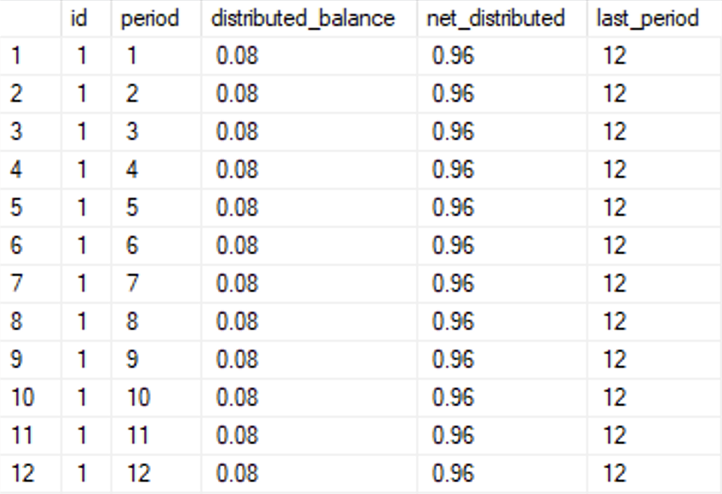
The correction that we want to add is the balance (1.00 in the screenshot) minus the distributed_balance, 0.96, and we want to add this correction only to the last row of each distribution, i.e. where period=last_period.

Using an inline CASE construct, that looks something like this:

WITH cte AS (
    SELECT bal.id,
           bal.balance,
           d.[period],
           CAST(bal.balance*d.[key] AS numeric(12, 2)) AS distributed_balance
    FROM #balances AS bal
    CROSS JOIN #distribution AS d
)

SELECT id, [period],
       distributed_balance
           +(CASE WHEN [period]=MAX([period]) OVER (PARTITION BY id)
                  THEN balance-SUM(distributed_balance) OVER (PARTITION BY id)
                  ELSE 0.0 END) AS distributed_balance
FROM cte;

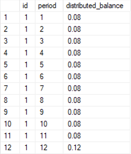
And here’s the result:

What about performance?

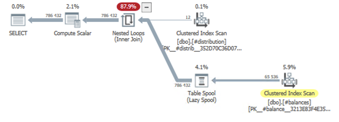
Obviously, the rounding error fix adds a lot of complexity to the query plan. Here’s the plan for the raw distribution:

When we apply the window functions required for our rounding fix, the plan grows:

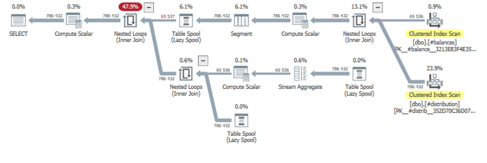
In the top-right corner, we still have the CROSS JOIN between #balances and #distribution. After that, we get a Segment operator which is used for our two window functions. The windowing itself happens in the following Table Spool and Nested Loops operators.

None of those two plans had any memory grant, because there was no sorting and no hashing going on. In a scenario with different distribution models, the CROSS JOIN would have been an INNER JOIN, and the plan would look different.

Other strategies

The optimization strategy will vary wildly between these types of scenarios, including to which row you’re adding the rounding errors. Astute readers may for instance have noted that in this particular example, the distribution table doesn’t add up to 100%, so you could try making a correction there first.

UPDATE d
SET [key]=[key]+correction
FROM (
    SELECT [key], (CASE WHEN [period]=MAX([period]) OVER ()
                        THEN 1.0-SUM([key]) OVER ()
                        ELSE 0 END) AS correction
    FROM #distribution
    ) AS d
WHERE correction!=0;

This won’t solve all of your rounding errors, but maybe some of them.