A very common challenge in T-SQL development is filtering a result so it only shows the last row in each group (partition, in this context). Typically, you’ll see these types of queries for SCD 2 dimension tables, where you only want the most recent version for each dimension member. With the introduction of windowed functions in SQL Server, there are a number of ways to do this, and you’ll see that performance can vary considerably.

On selectivity and density

When you’re working with grouping (and indexing, for that matter), you need to be aware of the density and selectivity of the table. These two metrics describe the uniqueness of the first key of an index. An index where the first key is near-unique has a low density and a high selectivity. The opposite is when the first key of an index only contains a few unique values in a table with lots of rows.

Example: an index on the social security number or birth date on a table of employees is fairly unique and has a very low density. An index on something like gender or age, on the other hand, will be highly dense.

The density of an index is reflected in the statistics and can greatly affect the efficiency of, or even the choice of query plan, and so you’ll see that different strategies perform differently depending on whether the table is dense or not.

Setting up the demo

Here is an example setup with two tables with 100 000 rows each. One table is dense and contains 10 partitions with about 10 000 rows each. The other is selective, containing about 33 000 partitions with only three rows each.

CREATE TABLE #dense (
    part    int NOT NULL,
    val     int NOT NULL,
    other   varchar(100) NOT NULL
);

CREATE CLUSTERED INDEX PK ON #dense (part, val);

INSERT INTO #dense (part, val, other)
SELECT TOP (100000)
    ROW_NUMBER() OVER (ORDER BY (SELECT NULL))/10000,
    ROW_NUMBER() OVER (ORDER BY (SELECT NULL))%10000,
    REPLICATE('x', 100)
FROM sys.columns AS c1
CROSS JOIN sys.columns AS c2
CROSS JOIN sys.columns AS c3;


CREATE TABLE #selective (
    part    int NOT NULL,
    val     int NOT NULL,
    other   varchar(100) NOT NULL
);

CREATE CLUSTERED INDEX PK ON #selective (part, val);

INSERT INTO #selective (part, val, other)
SELECT TOP (100000)
    ROW_NUMBER() OVER (ORDER BY (SELECT NULL))/3,
    ROW_NUMBER() OVER (ORDER BY (SELECT NULL))%3,
    REPLICATE('x', 100)
FROM sys.columns AS c1
CROSS JOIN sys.columns AS c2
CROSS JOIN sys.columns AS c3;

Apart from their contents, both tables have identical indexes, a clustered index on (part), our partitioning column, and (val), the ordering value.

Windowed MAX() function

SELECT *
FROM (
    SELECT *, MAX(val) OVER (PARTITION BY part) AS _max
    FROM #dense
    ) AS sub
WHERE val=_max;

In my opinion, this is a very intuitive strategy. The actual query plan, however has a surprise in store, mostly because we’re using an windowed function, which requires a table spool.

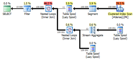
The plan is the same for the dense and the selective table, although the row estimates vary. For the dense table, this query completes in 800 ms, whereas the selective table takes about 1300 ms. The difference is the number of loops required for the Nested Loop operator – the fewer executions and more rows per execution, the faster.

ROW_NUMBER()

SELECT *
FROM (
    SELECT *, ROW_NUMBER() OVER (
        PARTITION BY part
        ORDER BY val DESC) AS _row_desc
    FROM #dense
    ) AS sub
WHERE _row_desc=1;

A similar approach uses a ROW_NUMBER() function instead of MAX(). That way, we can then filter out rows where the row number is 1. The downside is that this requires a different sort order for the ROW_NUMBER() function than that of the index, which results in a Sort operator.

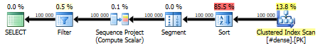
Sorts are expensive and blocking, so this query doesn’t really perform that well either. It is considerably faster than the MAX() solution, though, coming in at 300 ms for the dense table and 600 ms for the selective one.

Using LAST_VALUE()

SELECT *
FROM (
    SELECT *, LAST_VALUE(val) OVER (
        PARTITION BY part
        ORDER BY val
        ROWS BETWEEN CURRENT ROW AND UNBOUNDED FOLLOWING
        ) AS _max
    FROM #dense
    ) AS sub
WHERE val=_max;

You’d expect this one to be about equivalent to the MAX() solution, right? Actually, it shares more similarities with the ROW_NUMBER() strategy, because LAST_VALUE() is actually just FIRST_VALUE() with a reversed sort order. The query plan actually sorts the data stream by (part, val DESC), so the Sort operator makes this similarly expensive.

The dense query completes in about 500 ms and the selective one in 850 ms, which is even worse than ROW_NUMBER().

Using LEAD() to roll your own LAST_VALUE()

The trouble with MAX() and LAST_VALUE() is that they need to set up a window that spans all the way to the end of the partition, which could be thousands of rows forward in a dense table. When in fact, we only need to look if there is a next row in the same partition or not. If there isn’t, we can deduce that it must be the last row. This window only spans two rows – the current row and the next one.

SELECT *
FROM (
    SELECT *, (CASE WHEN LEAD(val, 1) OVER (
            PARTITION BY part
            ORDER BY val)
        IS NULL THEN 1 ELSE 0 END) AS _last
    FROM #dense
    ) AS sub
WHERE _last=1;

This solution is completely free of Sorts and other blocking operators. On the downside, the cardinality estimation gets lost on the way, which could hurt your plan if you plan to make this a subquery of something bigger.

As for performance, the dense query finishes in about 200 ms and the selective one in about 500 ms. This is our best performing solution so far.

CROSS APPLY with TOP 1

SELECT *
FROM (
    SELECT DISTINCT part
    FROM #dense) AS p
CROSS APPLY (
    SELECT TOP 1 d.*
    FROM #dense AS d
    WHERE d.part=p.part
    ORDER BY d.val DESC) AS x;

CROSS APPLY is an old favourite of mine, particularly as you can use it to force a Nested Loop. This is extremely efficient with dense tables, because every individual iteration is really fast, and the denser the table, the fewer the iterations.

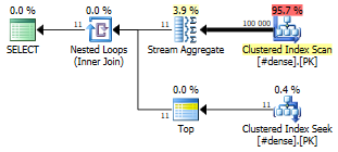
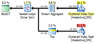
Note that the dense query (left) only has to perform 11 iterations. The selective table (right), on the other hand has 33 000 unique partitions to query. The former comes in at a lightning-fast 25 ms, the latter one finishes in about 750 ms, which is slower than most other alternatives.

Going old-school

This is how we used to do it before all of those fancy window functions that we’ve gotten so used to. It was simple and understandable.

SELECT d.*
FROM #dense AS d
INNER JOIN (
    SELECT part, MAX(val) AS _max
    FROM #dense
    GROUP BY part) AS x ON d.part=x.part AND
                           d.val=x._max;

The inner derived table (x) selects each partition and aggregates the maximum ordering value. Those two columns, the partition and the maximum ordering value, are then self-joined to the outer table (d). The query plan used to look something like this:

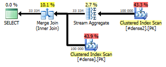
With an optimal index, you get Stream Aggregate and Merge Join, which are both exceptionally well-performing, non-blocking operators that don’t require a memory grant. But there’s still the self-join with a fairly large table.

But this is where the optimizer might throw you a little surprise: For some types of queries, it’ll short-cut your intended execution plan and completely redesign the plan to something much more efficient. This is one such query. Here’s what comes out instead:

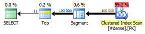
The Segment operator sets a flag whenever you enter/leave a partition, and the Top operator selects the first (TOP 1) row when that happens. It’s that simple. The dense query finishes in 25 ms, the selective one still takes about 500 ms.

TL;DR – conclusions

For this type of solution, a table with a dense index will return fewer rows, and in all of the strategies we’ve looked at, it performs faster than with a more selective index.

The CROSS APPLY and the old-school solutions are by far the best choice for dense indexes, i.e. when the first column has a low degree of uniqueness. The old-school solution is only that fast because the optimizer short-circuits the query plan.

LEAD() and the old school strategy are best for selective indexes, i.e. when the first column is highly unique.