At the November announcement of SQL Server 2025, a ton of cool new features were unveiled. It’s obviously very heavy on AI and Fabric, but those are the times we live in. If you squint a little, tough, you can make out quite a few really nice developer-centric features. And if you know anything about me, I’m a big fan of developer features and performance improvements.
Starting today, the public preview of SQL Server 2025 is available to download!
One really interesting new feature that got my attention was the addition of JSON indexes. I’m a big fan of everything that makes working with JSON easier, since JSON blobs are so much easier to work with than table variables when you’re moving data from point A to point B. This is especially true when you’re working with complex, relational data.
Disclaimer: While I’ve had access to a private preview of SQL Server 2025, I haven’t had a fully complete documentation to go by, nor have I bothered the folks working on the product with questions, so most of the following is my conjecture and may not even be true for the final product once it launches.
The syntax
Creating a JSON index is pretty straight-forward.
CREATE JSON INDEX name ON table_name (json_column_name)
[ FOR ( sql_json_path [,...n] ) ]
[ WITH ( <index_option> [,...n] ) ]
[ ON { filegroup_name
DEFAULT } ];
The FOR part works a little like the WHERE clause of a filtered index, but instead of filtering rows in the base table, it narrows the JSON index to specific JSON paths.
No huge surprises with the index options. You have your normal options, like DROP_EXISTING, ALLOW_PAGE_LOCKS, FILLFACTOR, PAD_INDEX, etc.
I found that the filegroup/data space assignment didn’t work yet in my private preview version. Using the “ON” clause just returns a syntax error. It appears that the JSON index data is always stored in the same file group or partition scheme as the base table.
How JSON indexes are stored
The JSON index data, unlike traditional rowstore or columnstore indexes, is not actually stored in a separate index on the table. It gets an entry in sys.indexes, but the rows are actually stored in an “internal table” (type=IT in sys.objects) in the database, and SQL Server keeps that internal table updated transparently and atomically, just like a regular rowstore index. This is similar to how XML indexes and spatial indexes work.
You can find this hidden table in two different ways:
- The name is sys.json_index_{object_id}_{index_id}, referring to the object id and index id of the JSON index.
- In sys.objects, the hidden table has a parent_object_id pointing to the base table
This architectural choice comes a couple of minor implications:
- Like any index, the hidden system table needs to be able to reference the base table, so unlike regular indexes, a heap or a clustered rowstore or columnstore index won’t suffice. The base table needs to have a clustered primary key.
- Determining the size of the base table using sys.dm_db_partition_stats won’t include the size of the internal table – you’ll specifically have to look at the internal table’s object_id in addition to that of the base table.
- In my testing, creating JSON indexes on temp tables was not allowed.
Regular database users can’t really look at the actual contents of an internal table object, but you can sneak a peek at it using a dedicated administrator connection (DAC).
--- Run in dedicated administrator connection:
SELECT TOP (1000) *
FROM sys.json_index_1150627142_1216000;
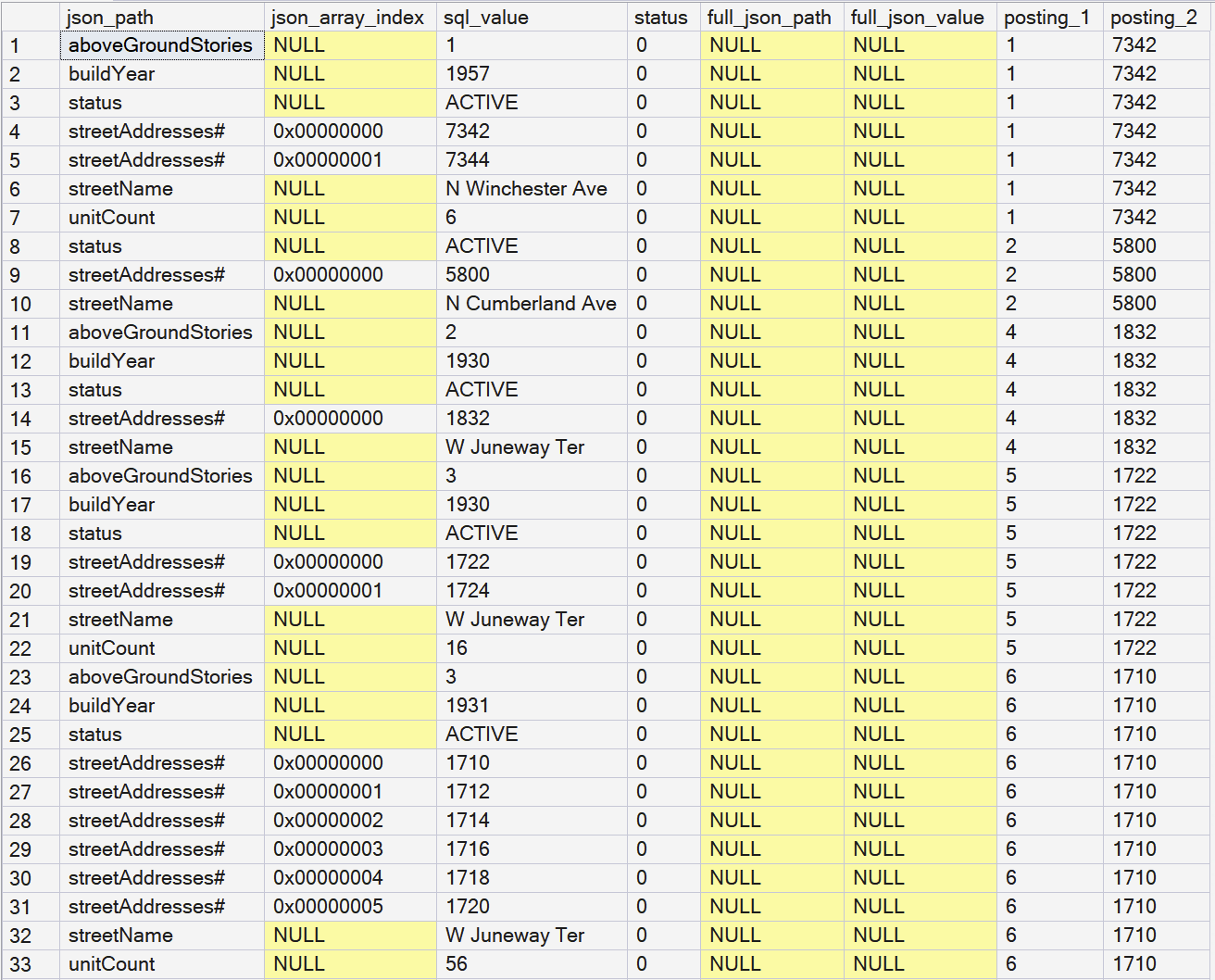
You can clearly see how the internal table contains a tabular representation of the JSON blob. Note how the “#” character along with json_array_index represents an array. For arrays-inside-arrays, the json_array_index will simply be twice the width, for example 0x0000000300000002 would be the second array member of the third array member.
The sql_value column is a sql_variant, in order to be able to store any type of data from the JSON blob. I have some thoughts on this, but I’m not going to play Monday-morning quarterback here.
Note the base table’s primary key columns, which are included as “posting_{1..n}”, in order to allow joins between the base table and the internal table.
Setting up some data
I found a suitable table in my Chicago Parking Tickets demo database to create some example data and try a few things out. The “Buildings” table contains about 488 000 rows and weighs in at about 300 MB uncompressed, as it also has a ton of spatial data in it.
I added a JSON column, populated the column with data from the row:
ALTER TABLE Chicago.Buildings ADD JSON_blob json NULL;

UPDATE b
SET b.JSON_blob=x.blob
FROM Chicago.Buildings AS b
CROSS APPLY (
    SELECT b.Street AS streetName,
           b.Building_Status AS [status],
           (SELECT JSON_ARRAYAGG(n.[value])
            FROM GENERATE_SERIES(b.From_Address, b.To_Address, CAST(2 AS smallint)) AS n
            ) AS streetAddresses,
           YEAR(b.Build_year) AS buildYear,
           NULLIF(b.Above_ground_stories, 0) AS aboveGroundStories,
           NULLIF(b.Below_ground_stories, 0) AS belowGroundStories,
           NULLIF(b.Number_of_units, 0) AS unitCount
    FOR JSON PATH, WITHOUT_ARRAY_WRAPPER
    ) AS x(blob);
All this JSON data roughly doubles the table size to about 600 MB. Here’s a rough idea of the JSON objects we’re creating, one building object per table row:
{"streetName": "N Winchester Ave",
 "status": "ACTIVE",
 "streetAddresses": [7342,7344],
 "buildYear": 1957,
 "aboveGroundStories": 1,
 "unitCount": 6
}

{"streetName": "N Cumberland Ave",
 "status": "ACTIVE",
 "streetAddresses": [5800]
}

{"streetName": "W Juneway Ter",
 "status": "ACTIVE",
 "streetAddresses": [1832],
 "buildYear": 1930,
 "aboveGroundStories": 2
}
Note how a building can have multiple street addresses (numbers), so we’re assigning those to an array.
Without a JSON index
Let’s first set a benchmark and see what kind of performance we get without a JSON index, with a couple of test queries:
Query 1, no index
First, let’s see if we can locate the iconic Rookery building, a Chicago landmark with a lobby renovated by none other than Frank Lloyd Wright, and featured in the movie The Untouchables as the headquarters of the Chicago PD.
SELECT Building_ID, JSON_blob
FROM Chicago.Buildings
WHERE JSON_VALUE(JSON_blob, '$.streetName')='S La Salle St'
  AND JSON_VALUE(JSON_blob, '$.streetAddresses[0]')<=209
  AND JSON_VALUE(JSON_blob, '$.streetAddresses[last]')>=209;
The execution plan doesn’t hold any surprises. Because there’s no index on the contents of the JSON column, we need to scan and check each and every row of our 622 MB table.
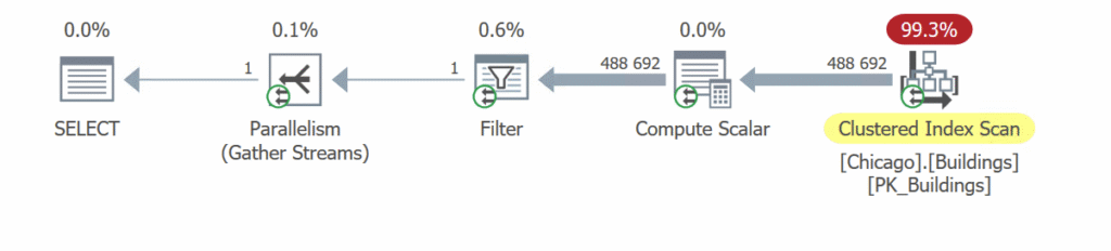
The Compute Scalar parses the JSON object, the Filter subsequently checks the results and keeps only the row(s) we want. This query runs for 1450 ms of CPU time (700 ms execution time) with 79 416 reads on the base table.
Query 2, no index
Let’s try the same query with the JSON_CONTAINS function, which is new for SQL Server 2025.
SELECT Building_ID, JSON_blob
FROM Chicago.Buildings --WITH (INDEX=IX_JSON)
WHERE JSON_CONTAINS(JSON_blob, 'S La Salle St', '$.streetName')=1
  AND JSON_CONTAINS(JSON_blob, 209, '$.streetAddresses[*]')=1;
The query plan looks exactly the same, the reads are roughly similar, but the execution time has gone up to 2400 ms CPU time (1240 ms execution time).
Still, JSON_CONTAINS is a much better choice for this particular dataset and query, because we don’t really want to rely on the “streetAddresses” array being ordered.
As expected, without a JSON index, there’s really no practical way to avoid scanning the entire base table (unless we invent our own JSON index logic with parsing logic and indexed, computed columns, but that’s a blog post for another year).
With a JSON index
CREATE JSON INDEX IX_JSON
   ON Chicago.Buildings (JSON_blob)
   FOR ('$')
   WITH (DATA_COMPRESSION=PAGE);
The new JSON index adds 45 MB (page compressed) + 150 MB (uncompressed) to the database. If we want it smaller, we can use the FOR clause to isolate just the JSON paths we’re interested in.
CREATE JSON INDEX IX_JSON
   ON Chicago.Buildings (JSON_blob)
   FOR ('$.streetName', '$.streetAddresses')
   WITH (DATA_COMPRESSION=PAGE, DROP_EXISTING=ON);
This reduces the index to just 17+65 MB is size.
Now, let’s run the same queries again.
Query 1, with JSON index
I’ve replaced the columns with a plain COUNT(*) in order to try to make the JSON index covering, but no luck: the base table invariably gets up being joined in. This isn’t a big deal for single-row type results, but it could spell trouble for larger workloads.
SELECT COUNT(*) -- Building_ID, JSON_blob
FROM Chicago.Buildings
WHERE JSON_VALUE(JSON_blob, '$.streetName')='S La Salle St'
  AND JSON_VALUE(JSON_blob, '$.streetAddresses[0]')<=209
  AND JSON_VALUE(JSON_blob, '$.streetAddresses[last]')>=209;
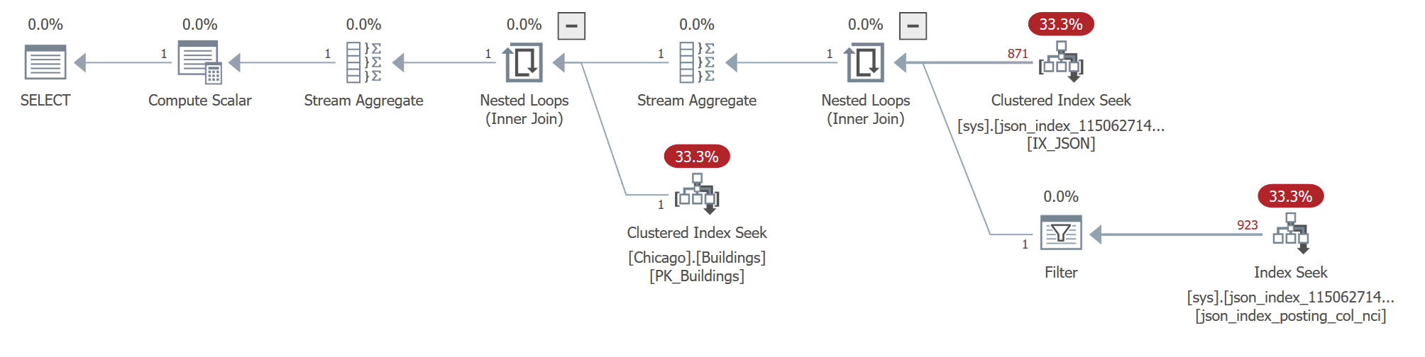
Note how the two Seek operators (the “streetName” and “streetAddresses” criteria, respectively) now use the internal table, sys.json_index_1150627142_1216000, instead of the base table:
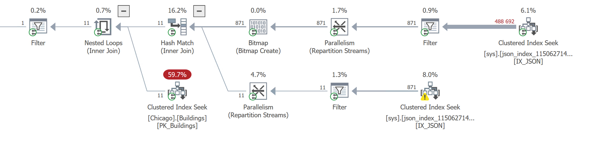
This query runs for 470 ms CPU (234 ms duration), which is about three times as fast as it did before. It performs 2000 reads on the JSON index and just 40 reads on the base table, which is a big improvement, compared to scanning the entire 600 MB base table.
The top branch, the streetAddress, collects 871 matching rows. Here, the optimizer chooses to use a “Bitmap” using the primary key columns from the base table, which it then applies to the lower branch’s Clustered Index Seek, in order to fetch just those 871 rows from the base table. Originally designed for star schema-type lookups, I love the Bitmap operator specifically because it can help out with these types of optimizations.
But there’s a reason we had to resort to a Bitmap. Take another look at the top-right Clustered Index Seek. We’re actually reading all streetName values in the entire City of Chicago, and then filtering for S La Salle Street.
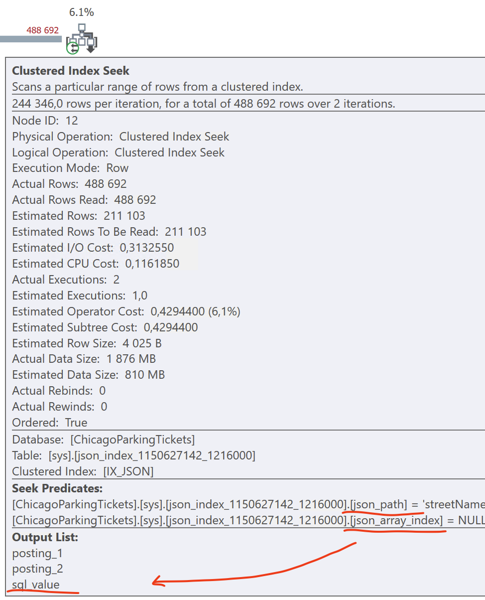
For some reason, the Seek predicate does not filter on the street name (i.e. the “sql_value” column), even though it is in the clustered index on the internal table. Here, the optimizer should have looked for three, not two, equality criteria: on the (json_path, json_array_index, sql_value) columns, rather than just (json_path, json_array_index).
I have no idea if this is a bug or feature, or if it will change in the release version. I imagine that indexing a sql_variant column can be really tricky to implement in the engine.
Query 2, with JSON index
But enough with the needlessly complicated JSON_VALUE construct, which isn’t a great fit to find values in an array. Let’s try the JSON_CONTAINS query with the new shiny index, and see how it does:
SELECT COUNT(*) -- Building_ID, JSON_blob
FROM Chicago.Buildings --WITH (INDEX=IX_JSON)
WHERE JSON_CONTAINS(JSON_blob, 'S La Salle St', '$.streetName')=1
  AND JSON_CONTAINS(JSON_blob, 209, '$.streetAddresses[*]')=1;
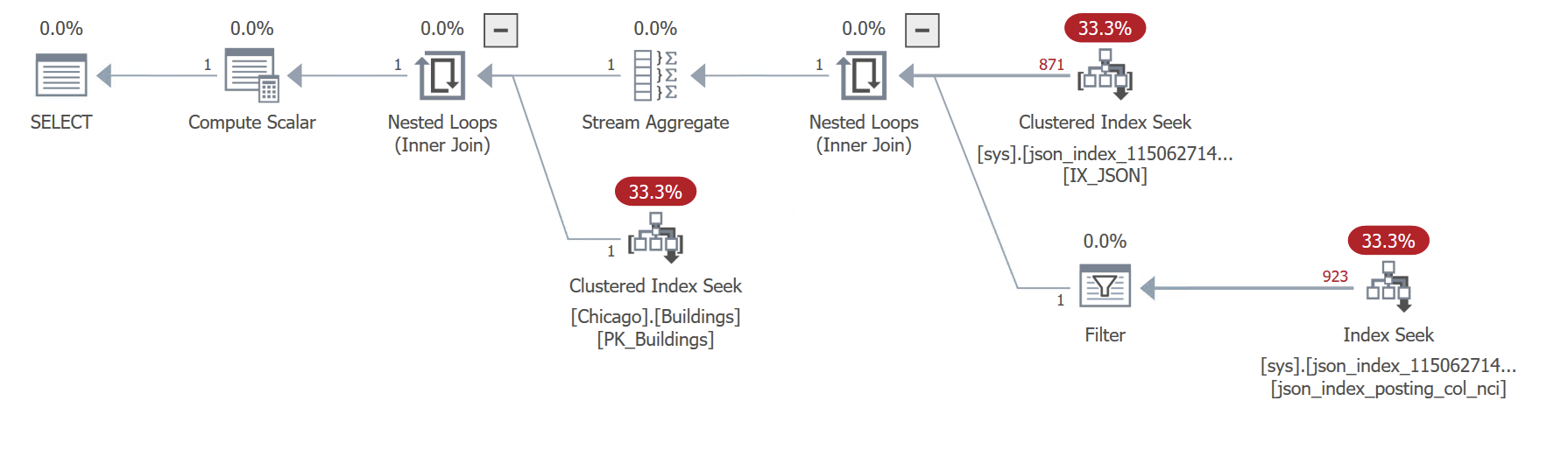
For the first time, we get a serial plan, because the query is now so light-weight and fast. It runs for just 6 ms of execution time, with hardly any CPU time at all. The JSON index gets 2636 reads, which is slightly higher than Query 1, and the base table gets only 3 reads, for the exact row we’re returning.
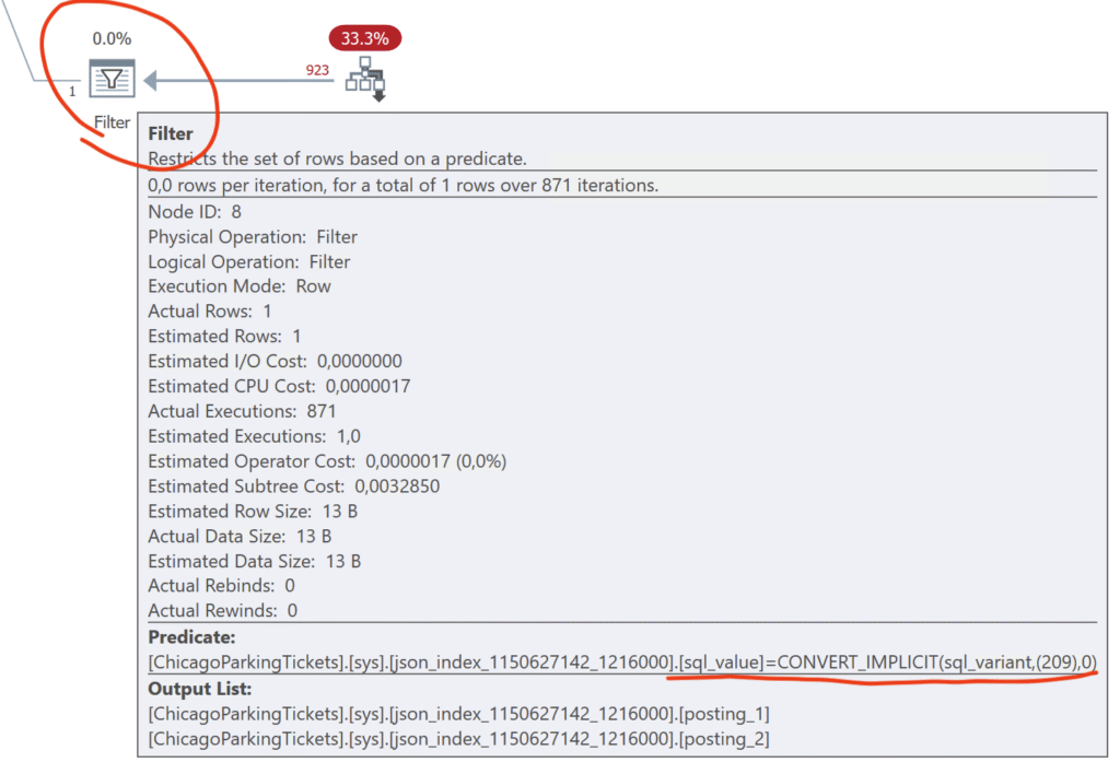
But like we saw in Query 1, for some reason, the lower-right Seek can’t seem to seek the precise key value (209) that we’re looking for, so this is delegated to a subsequent Filter operator. I guess it doesn’t make much difference in this case, but it still feels a little strange.
Early teething problems
DATA_COMPRESSION only compresses the clustered index on the internal table, but not the non-clustered index for some reason.
Each column can only have a single JSON index. While I don’t think this is a design limitation (clearly, the data model would support multiple indexes), maybe getting the optimizer to choose the correct index might be a nightmare.
I’m looking forward to file groups, partitioning, all that jazz, which I’m sure will get added in due time before release.
JSON indexes are not covering, even when they are
But the most confounding thing I found was that there’s no apparent way to use a JSON index as a covering index, where the index itself contains all the information you need to process the query. Every execution plan I’ve seen so far will always join back to the base table in the end.
Check out this example:
SELECT JSON_VALUE(JSON_blob, '$.streetName') AS streetName,
       JSON_VALUE(JSON_blob, '$.streetAddresses[0]') AS streetAddress_first,
       JSON_VALUE(JSON_blob, '$.streetAddresses[last]') AS streetAddress_last
FROM Chicago.Buildings --WITH (INDEX=IX_JSON)
WHERE JSON_CONTAINS(JSON_blob, 'S La Salle St', '$.streetName')=1
  AND JSON_CONTAINS(JSON_blob, 209, '$.streetAddresses[*]')=1;
Note how we’re filtering on streetName and streetAddresses, so we’re already reading that data from the JSON index. But when we try to display those two columns using JSON_VALUE, it reads the actual JSON blob from the base table, and then computes the JSON_VALUE from that.
Note the Compute Scalar in the top-left corner, which performs the JSON_VALUE on data collected from the base table’s JSON blob.
Conclusion
I was expecting JSON indexes to be just opaque database pages in yet another type of index, but I was kind of delighted to find, almost by accident, that I could actually go and look for myself “how the sausage is made”. As rowstore indexes have done for half a century now, I’m very happy to see JSON indexes eliminating the need to scan large tables from end to end, and instead being able to Seek to the exact rows we’re looking for.
Because of this, and with a little luck, SQL Server should be able to leverage the decades of hard work that has gone into things like good cardinality estimations and optimizations, rather than having to reinvent a lot of wheels.
Sure, if you’re just bulk loading JSON blobs as part of your ETL process, this might not make much of a difference to you. But if the data stays in JSON, and you’re using that JSON column to store (and query) unstructured data in your app, this is a huge improvement.
And combined with the addition of sp_invoke_external_rest_endpoint to SQL Server, being able to fetch datasets from HTTP endpoints, I think a lot of ETL work just became orders of magnitudes simpler and faster.
I’m a fan.
Nice article, thank You for it!