As you could read in the indexing basics article, a well-defined index can boost query performance, but there are a few more basic tricks that can have a great impact on how your query is executed. One of the most important is a technique called covering indexes. A covering index is basically a non-clustered index that covers all the columns you need in a query, not just the keys.
A quick re-cap on non-clustered indexes
Non-clustered indexes are organized the same way as clustered indexes, except the leaf nodes of a clustered index contains the actual table data. The leaf nodes of non-clustered indexes contain only pointers to where the row data is stored. This could be a row (a RID) in a heap or a leaf node of a clustered index (a clustering key).
Key lookups and RID lookups
If your query uses an index that contains the key columns a and b, but your query also needs the c column of the table, the query plan will need to “join” the index data (which contains a and b) to the underlying heap or table, in order to get to c. In the query plan, this “join” is called a RID lookup if it’s a heap, or a Key lookup if the table has a clustered index.
This may sound complicated, but the following example will hopefully make it really easy to understand.
Example
Let’s say we have a table that looks like this:
CREATE TABLE #test (
    a    int NOT NULL,
    b    int NOT NULL,
    c    int NOT NULL,
    amount    numeric(18, 2) NOT NULL
)

CREATE UNIQUE CLUSTERED INDEX #test_ix1 ON #test (a)

INSERT INTO #test (a, b, c, amount)
SELECT 1, 1001, 2001, 1234.56 UNION ALL
SELECT 2, 1002, 2002, 2234.56 UNION ALL
SELECT 3, 1003, 2003, 3234.56 UNION ALL
SELECT 4, 1004, 2004, 4234.56 UNION ALL
SELECT 5, 1005, 2005, 5234.56 UNION ALL
SELECT 6, 1006, 2006, 6234.56 UNION ALL
SELECT 7, 1007, 2007, 7234.56 UNION ALL
SELECT 8, 1008, 2008, 8234.56 UNION ALL
SELECT 9, 1009, 2009, 9234.56
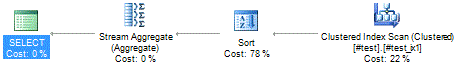
Let’s look at the different query plans that the following query will generate:
SELECT c, SUM(amount) AS amount_aggregate
FROM #test
WHERE b>=2004 AND b<2007
GROUP BY c
With just the basic clustered index in the example above, this query will scan through the clustered index.
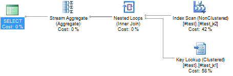
If we add an extra non-clustered index on the c column..
CREATE INDEX #test_ix2 ON #test (c)
.. the query plan will start using this index. However, if we use the #test_ix2 index, we’ll have to look up the b and amount columns that aren’t indexes. That’s what the “Key lookup” in the lower-right corner does, it joins the leaf nodes of the table (#test_ix1) to the index (#test_ix2).
This can be a potentially very expensive operation. The way to avoid this is to make the b and amount columns available in the index, so the database engine won’t have to go hunting for them in the clustered index. This is done with the INCLUDE clause of the CREATE INDEX statement:
DROP INDEX #test.#test_ix2

CREATE INDEX #test_ix2 ON #test (c) INCLUDE (b, amount)
Now, when you run the same query, the execution plan will look like this:
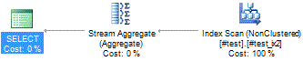 As you can see from the query plan, the entire query is performed using only the non-clustered index on the table, because this index has all the data that we need to complete the query.
Sort orders on non-clustered covering indexes
A non-clustered index designed as a covering index for a query acts a bit like a separate table, and by separate, I mean that it has all the data you need stored in the index, and much like a clustered index, you define the column order and the sort order of those columns in the index.
This means that if you’re trying to optimize a particularly tricky JOIN query, you can add a covering index to help speed up the data query, but you can also add just the right sort order for your query, so you’ll hopefully end up with a super-efficient join that will speed up your query.
8 comments