The SQL Server query optimizer can find interesting ways to tackle seemingly simple operations that can be hard to optimize. Consider the following query on a table with two indexes, one on (a), the other on (b):

SELECT a, b
FROM #data
WHERE a<=10 OR b<=10000;

The basic problem is that we would really want to use both indexes in a single query.

In this post, we’re going to take a look at a few examples of how this type of query would be optimized, as well as how statistics can affect the query plan, and finally, we’ll take a look at a slightly rare plan operator called “Merge Join (Concatenation)”.

Some test data

Let’s start by setting up a temp table with 100 000 dummy rows. To make the table a bit larger, I’ve added a “blob” column, so each rows is roughly 908 bytes wide. It’ll end up just shy of 100 MB, but if you’re short on space, feel free to eliminate the blob column.

CREATE TABLE #data (
    a           int NOT NULL,
    b           int NOT NULL,
    blob        char(900) NOT NULL
);

--- A clustered index on (a) and a non-clustered index on (b)
CREATE UNIQUE CLUSTERED INDEX #PK_data ON #data (a);
CREATE UNIQUE INDEX #IX_data ON #data (b) INCLUDE (blob);

--- Add 100 000 rows to the table:
INSERT INTO #data (a, b, blob)
SELECT TOP 100000
       ROW_NUMBER() OVER (ORDER BY (SELECT NULL)) AS a,
       100000-ROW_NUMBER() OVER (ORDER BY (SELECT NULL)) AS b,
       REPLICATE('xyz', 300) AS blob
FROM sys.columns AS c1
CROSS JOIN sys.columns AS c2;

The table is going to contain 100 000 rows, where column a goes from 1 to 100 000 in ascending order, while column b goes from 99 999 to 0 in descending order.

Now for some test queries:

Query 1

SELECT a, b, blob
FROM #data
WHERE a<=90000 OR b<=9000;

This query selects nearly every row in the table, because the first criteria (a<=90000) selects the first 90 000 rows and the second criteria (b<=9000) selects the last 9000 rows. Returning literally 99% of the table means that a single Index Scan with just an additional Filter to eliminate the 1% will suffice:

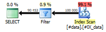
This query is completely non-blocking and requires no memory grant, but it needs to scan the entire table.

Query 2

Let’s change things. Narrowing down the selection on the two columns makes the previous plan rather wasteful – after all, if you just want 10% of the table, why scan the whole thing?

SELECT a, b
FROM #data
WHERE a<=10 OR b<=9000;

Note that with this query, we actually have two different index choices to consider: First off, selecting rows where (a<=10) is best left to the clustered index, because it indexes (a). The second part of the WHERE clause is a lot better suited for the non-clustered index on (b). Can we combine two indexes on the same table in the same query? Turns out, we can:

What the query optimizer basically does is optimize the query into this:

--- Pseudo T-SQL:
SELECT DISTINCT a, b
FROM (
    SELECT a, b
    FROM #data
    WHERE a<=10

    UNION ALL

    SELECT a, b
    FROM #data
    WHERE b<=9000
) AS sub;

.. although these two technically won’t generate the same plan.

So while we would assume that a WHERE clause on a single table would use a single Index Scan, in practice, it can be optimized to use two Index Seeks that each are a lot more efficient, and then concatenate (union) those two streams together and aggregate them to make them distinct.

Note the Hash Match (Aggregate) operator, which is blocking – it has to build hash tables, which means it has to consume the entire input before it starts spitting out results, and it has to allocate a bit of memory to do that.

Query 3

The third example looks like this:

SELECT a, b
FROM #data
WHERE a<=10000 OR b<=10;

This query will result in the following plan:

Note that this plan looks similar to the previous plan – it seeks on two indexes, concatenates them and makes the result distinct using an aggregate. In this case, the query plan sorts the input stream from the non-clustered Index Seek, which enables it to concatenate two identically ordered streams. The Merge Join (Concatenation) and Stream Aggregate operators both require the stream to be properly sorted, but on the other hand, they are non-blocking, i.e. they don’t require a memory grant and are very efficient.

This query will still require a small memory grant, but we only expect to see 11 rows from the non-clustered Index Seek, so we’ll just sort those rows at near-zero cost and memory grant.

Statistics

There’s no magic to choosing the right plan for the a query. The trick is knowing (estimating, really) how many rows each criteria will generate.

Statistics on the two indexes can give reasonably accurate estimates of the number of rows we’re likely to encounter. For instance, the statistics can tell us that there are somewhere in the range of 10 rows with (a<=10) and about 9001 rows where (b<=9000). In practice, statistics are not very fine-grained, and if you look again at the plan for Query 2, the estimate for the a column was really 2 rows, not the actual 10. However, statistics are not meant to be precise, only to give help generating a reasonably optimal plan for each query.