Today, we’re going to be looking at a kind of poor-mans’s-partitioning, using a view to union records from multiple tables. We’ll also take a look at when you would want this type of solution, some benefits and drawbacks, as well as ways to make things go faster.

On table partitioning

Partitioning a table effectively splits the contents of the table into multiple “tables” known as partitions (which are not transparent to users). The main advantage of partitioning is that you can store different parts of your data on different physical units, using filegroups. You can also switch data in and out of a partitioned table, which is very desirable in many datawarehouse applications.

For instance, you can store old data that isn’t referenced very often on slower drives, or perhaps on drives that have better read performance and less write performance (since this data doesn’t change), whereas you can keep your current data on drives with good overall read/write performance.

Partitioning in SQL Server, however, is an Enterprise Edition feature, and as such, may not be available to you if you haven’t got the budget.

Partitioned views

Luckily, you can create your own partitioning. It isn’t quite as flexible, but it can be just as powerful if you know what you’re doing. Microsoft calls this partitioned views. In essence, you have to manually design tables that represent each “partition”, and then bunch all those tables together using UNION ALL operators in a view. This view is your “partitioned view”, and it works in many ways like a partitioned table would.

Here’s an example of a very basic partitioned view. It partitions sales facts into three different tables. One table holds data for the current month, one for the current year (except the current month) and the thirds holds history facts, i.e. for previous years.

--- History
CREATE TABLE FACT.sales_history (
    [date]    date NOT NULL,
    dim1      int NOT NULL,
    dim2      int NOT NULL,
    dim3      int NOT NULL,
    dim4      int NOT NULL,
    amount1   numeric(10, 2) NOT NULL,
    amount2   numeric(10, 2) NOT NULL,
    CONSTRAINT PK_sales_history
        PRIMARY KEY CLUSTERED ([date], dim1, dim2, dim3, dim4)
) ON [PRIMARY];

--- Current year
CREATE TABLE FACT.sales_thisyear (
    [date]    date NOT NULL,
    dim1      int NOT NULL,
    dim2      int NOT NULL,
    dim3      int NOT NULL,
    dim4      int NOT NULL,
    amount1   numeric(10, 2) NOT NULL,
    amount2   numeric(10, 2) NOT NULL,
    CONSTRAINT PK_sales_thisyear
        PRIMARY KEY CLUSTERED ([date], dim1, dim2, dim3, dim4)
) ON [PRIMARY];

--- Current month
CREATE TABLE FACT.sales_thismonth (
    [date]    date NOT NULL,
    dim1      int NOT NULL,
    dim2      int NOT NULL,
    dim3      int NOT NULL,
    dim4      int NOT NULL,
    amount1   numeric(10, 2) NOT NULL,
    amount2   numeric(10, 2) NOT NULL,
    CONSTRAINT PK_sales_thismonth
        PRIMARY KEY CLUSTERED ([date], dim1, dim2, dim3, dim4)
) ON [PRIMARY];

With this solution, you can define a file group for each table, just like you would assign file groups to partitions. In this example, I’ve put all three tables in the PRIMARY filegroup. Rounding off the creation is a view that unions all these tables:

CREATE VIEW FACT.sales
WITH SCHEMABINDING
AS

SELECT [date], dim1, dim2, dim3, dim4, amount1, amount2
FROM FACT.sales_history
UNION ALL
SELECT [date], dim1, dim2, dim3, dim4, amount1, amount2
FROM FACT.sales_thisyear
UNION ALL
SELECT [date], dim1, dim2, dim3, dim4, amount1, amount2
FROM FACT.sales_thismonth

GO

Ok, those are the basics, but you’ll need a few more things to make this run smoothly.

CHECK constraints

For this to be a partitioned view and not just a bunch of tables with UNION ALLs between, you’ll need to define what’s in each table. If you were to compare this solution to a partitioned table, you’d already have the partition scheme in place (which tables hold the data, and what file groups those tables reside on), but no partition function (i.e. which partition contains what data). We’re going to need some way of determining which data goes in what base table.

This is done using CHECK constraints. Like the name implies, they are constraint mechanisms that enforce a certain business logic on each row in the table. But the SQL Server query optimizer also uses these constraints to improve queries, because they provide hints of what kind of data is stored in the table. In this case, we want to make sure that for instance the fact_thismonth table only contains data for the current month.

Here are some check constraints that we’re going to apply to the table.

--- History table contains 2013 and backward:
ALTER TABLE FACT.sales_history
    ADD CONSTRAINT CHK_sales_history_date
        CHECK ([date]<{d '2014-01-01'});

--- "This year" is data from 2014, but prior to august.
ALTER TABLE FACT.sales_thisyear
    ADD CONSTRAINT CHK_sales_thisyear_date
        CHECK ([date]>={d '2014-01-01'} AND [date]<{d '2014-08-01'});

--- "This month" is data from august 2014.
ALTER TABLE FACT.sales_thismonth
    ADD CONSTRAINT CHK_sales_thismonth_date
        CHECK ([date]>={d '2014-08-01'} AND [date]<{d '2014-09-01'});

If you were to run the following example SELECT query on the partitioned view before and after we’ve put these check constraints in place, you would get two radically different query plans.

SELECT *
FROM FACT.sales
WHERE [date]={d '2014-03-14'};

Without the check constraints:

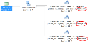
… and with the check constraints:

See what just happened? Using the check constraints, SQL Server can determine that the data we’re looking for can only exist in one of the tables. The performance impact from this difference in query plan can be considerable, particularly if the history table contains millions of rows.

Moving data in and out of “partitions”

Partition views, like other simple views, are updatable. If you perform updates on a “partitioning column”, i.e. a column that we’ve defined in the check constraints above, SQL Server will actually move the affected rows from one table to another when neccessary. Contrary to the example above, I would recommend you to always keep open intervals in your check constraints: In the example, the “current month” will contain any data starting with august 1, 2014 and ending on august 31. If for some reason, you were to create rows dated later than that, there wouldn’t be a table that could hold those rows, and you’d get the following error:

Msg 4457, Level 16, State 1, Line 1
The attempted insert or update of the partitioned view failed because the value of the partitioning column does not belong to any of the partitions.

To prevent this problem, make sure you use an open interval on both the lower and the upper boundaries of the partitions in order to allow storage of any valid value. In this case, you could change the constraint for the “current month” table to:

--- "This month" is data from august 2014.
ALTER TABLE FACT.sales_thismonth
 ADD CONSTRAINT CHK_sales_thismonth_date
        CHECK ([date]>={d '2014-08-01'} /* AND [date]<{d '2014-09-01'} */ );

Sargability

A while ago, I wrote a post about sargability. In short, what applies to index seeks and scans in terms of sargability, also applies to check constraints, and thus also to partitioned views. The following two queries will yield two different query plans, but they will return exactly the same data.

This query doesn’t use a sargable criteria:

SELECT * FROM FACT.sales
WHERE DATEPART(mm, [date])=3;

… while this one does:

SELECT * FROM FACT.sales
WHERE [date]>={d '2014-03-01'} AND [date]<{d '2014-04-01'};

The difference is that the first query uses a function to evaluate each row from FACT.sales. The second query, on the other hand, scans a specific range of values in FACT.sales, and that’s where the query optimizer can identify one underlying table (you could call this partition elimination).

Understanding sargability is an important concept in performance tuning, and this goes for partitioned views as well.

Redefining “partitions” by changing the constraints

In order to change the very definition of your partition boundaries, you need to change the CHECK constraints. Bear in mind, though, that this will not automatically move any data between the table. In order to accomplish this, you’ll need to do a bit of manual work.

Here’s an idea on how to change the “current month” partition from august 2014 to september 2014:

BEGIN TRANSACTION;

    --- Drop the old constraint for "this year":
    ALTER TABLE FACT.sales_thisyear
        DROP CONSTRAINT CHK_sales_thisyear_date;

    --- Drop the old constraint on "this month":
    ALTER TABLE FACT.sales_thismonth
        DROP CONSTRAINT CHK_sales_thismonth_date;

    --- Create the new constraint for "this year"
    --- in order to allow the new values:
    ALTER TABLE FACT.sales_thisyear
        ADD CONSTRAINT CHK_sales_thisyear_date
            CHECK ([date]>={d '2014-01-01'} AND [date]<{d '2014-09-01'});

    --- Add data from "this month" to "this year":
    INSERT INTO FACT.sales_thisyear
    SELECT *
    FROM FACT.sales_thismonth;

    --- Clear the contents of "this month":
    TRUNCATE TABLE FACT.sales_thismonth;

    --- Re-apply the check constraint on "this month",
    --- but for september instead:
    ALTER TABLE FACT.sales_thismonth
        ADD CONSTRAINT CHK_sales_thismonth_date
            CHECK ([date]>={d '2014-09-01'});

COMMIT TRANSACTION;

Incidentally, dropping the check constraints in the beginning of the transaction creates an exclusive schema lock on these two tables, preventing other processes from performing any operations on the data until we’ve committed the transaction – this is just what we want.

Other advantages to partitioned views

We’ve spent some time looking at why partitioned views are a “poor man’s partitioning”, and how regular partitioning can be superior, but there are a few cases where partitioned views are actually more powerful.

Partitioned views can share “partitions” (the underlying tables) between them. This may be an advantage in some specific implementation.

If you really put some effort into it, you can design partitioned views that span multiple servers – this is done using linked servers, where the base tables are spread out on different SQL Server machines. This is called a distributed partitioned view, and it is a bit tricker to design and maintain.

That’s it for this week! Check back next week for more T-SQL goodies. And don’t forget to subscribe to this blog and like the Sunday Morning T-SQL Facebook page!